Fine-Tuning a Local LLM Judge with WANDS and Qwen

I wanted to know whether a local LLM could act as a useful search relevance judge.

This post is for people considering LLM-as-judge workflows for search, retrieval, or relevance grading. It is not a recipe for magically turning a small model into a human replacement. It is a case study in what happens when you actually try to do the whole thing: data prep, training, local inference, hosted-model comparison, and error analysis.

Why I did this

I wanted to write a small case study for judgement-ai, my open-source pipeline for grading search results with LLMs. The idea behind the tool is simple: take query-document pairs, send them to a local or hosted model, ask for a structured relevance score, and save the judgments in a format that can be compared later.

WANDS was a good dataset for this because it is public, MIT-licensed, and built specifically for product search relevance. It already has human labels for query-product pairs, so I could use it to check whether LLM-generated judgments matched an existing human benchmark.

This turned into a longer project than I expected. I prepared the dataset, built a benchmark split, fine-tuned a local Qwen model, ran the benchmark through judgement-ai, and then compared the local model against GPT-5.5 and an instruct Qwen baseline. The result was mixed: the fine-tuned local model improved, GPT-5.5 was still much stronger, and the whole process made it obvious that fine-tuning a useful judge is not a quick weekend task.

There are many knobs: the dataset split, label balance, base model, prompt format, context length, learning rate, number of epochs, adapter settings, and evaluation metric. With limited compute, every choice feels expensive. That is the real reason this post is long. In addition to the final score table, I will present the full path from raw relevance data to a judged benchmark, including where the local model did and did not improve.

The short version: the local fine-tuned model became more useful, but not good enough to replace human judges. The evaluation loop was the valuable part.

Preparing WANDS for LLM relevance judging

Before benchmarking any models, I needed to turn WANDS into the kind of input my judging pipeline could handle.

WANDS is Wayfair’s product search relevance dataset. It was published with the ECIR 2022 paper WANDS: Dataset for Product Search Relevance Assessment and contains product search queries, product metadata, and human relevance labels for query-product pairs.¹ Each label describes whether a candidate product is an Exact, Partial, or Irrelevant match for a query.²

The raw dataset is organized around three pieces of information: search queries, products, and human relevance labels. I joined these into a single query-product-label table where each row represented one product candidate for one search query.

For the LLM input, I kept the fields that looked directly useful for relevance judging:

• the search query
• product name
• product class
• category hierarchy
• product description

I removed fields like product ratings and review counts. Those fields may be useful for ranking products, but they are not direct evidence that a product matches a query.

Table 1. Joined WANDS row

Field	Value
query_id	15
product_id	39828
label	Irrelevant
score	0
query	black 5 drawer dresser by guilford
product_name	fairlin 5 drawer storage cabinet
product_class	Office Storage Cabinets
category_hierarchy	Furniture / Office Furniture / Office Storage Cabinets

Product description excerpt:

the features never stop unfolding with this multifunctional storage hutch…

Table 1. A single benchmark row after joining the WANDS query, product, and label tables. Each row becomes a query-product relevance judgment.

The original WANDS label strings were converted into numeric scores:

WANDS label	Score
Irrelevant	0
Partial	1
Exact	2

The original usable label distribution was not balanced after joining and filtering the data:

Table 2. Original usable WANDS label distribution after joining and filtering

WANDS label	Share of usable rows
Partial	63.0%
Irrelevant	26.0%
Exact	11.0%

This mattered because a purely random sample would mostly produce Partial examples and relatively few Exact examples. Since I wanted to evaluate whether models could tell all three relevance levels apart, I needed a more diagnostic benchmark split later.

This matched the output format expected by my judging pipeline. During training and benchmarking, models were asked to return only one of:

SCORE: 0
SCORE: 1
SCORE: 2

The exported instruction-tuning rows contained an instruction, an input block, and a target output. The input block included the query and product details, while the output contained only the score.

Table 3. Example instruction-tuning row

{
  "query_id": 15,
  "product_id": 39828,
  "instruction": "Given a search query and a candidate product, predict the relevance score...",
  "input": {
    "query": "black 5 drawer dresser by guilford",
    "product_name": "fairlin 5 drawer storage cabinet",
    "product_class": "Office Storage Cabinets",
    "category_hierarchy": "Furniture / Office Furniture / Office Storage Cabinets",
    "product_description": "the features never stop unfolding with this multifunctional storage hutch..."
  },
  "output": "SCORE: 0"
}

Table 3. Example instruction-tuning row. The model receives query and product fields, then learns to return a score-only judgment. Note that the actual JSONL file concatenates the input attributes into a single prompt string.

Building the benchmark set

I did not use a purely random benchmark split. Random sampling would have made the benchmark easier to create, but less useful for diagnosis.

Instead, I built a controlled benchmark set:

• 50 held-out queries
• 10 products per query
• 500 total query-product pairs
• each benchmark query included at least two Exact, two Partial, and two Irrelevant examples

This made the benchmark more balanced than the natural WANDS distribution. A random sample would have produced fewer Exact examples and made it harder to inspect where models failed. I wanted a benchmark where every model had to distinguish between all three relevance levels.

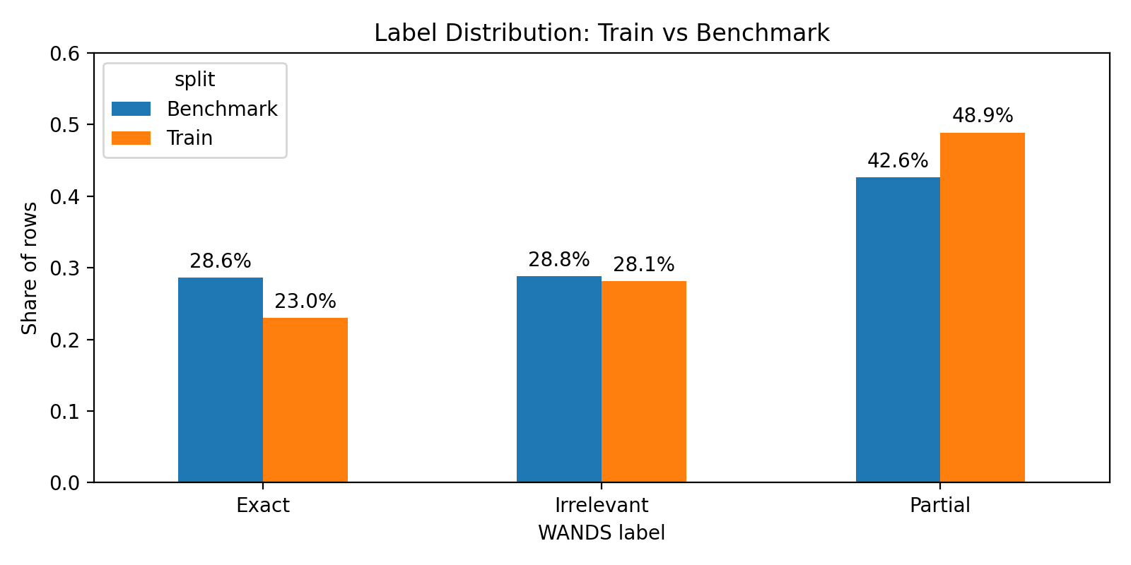
Figure 1. Label distribution in the training and benchmark sets. The benchmark was more balanced so that model behavior on all three labels could be inspected.

The benchmark was also structured by query. Each query contributed 10 products, which made it easier to compare model behavior across different search intents.

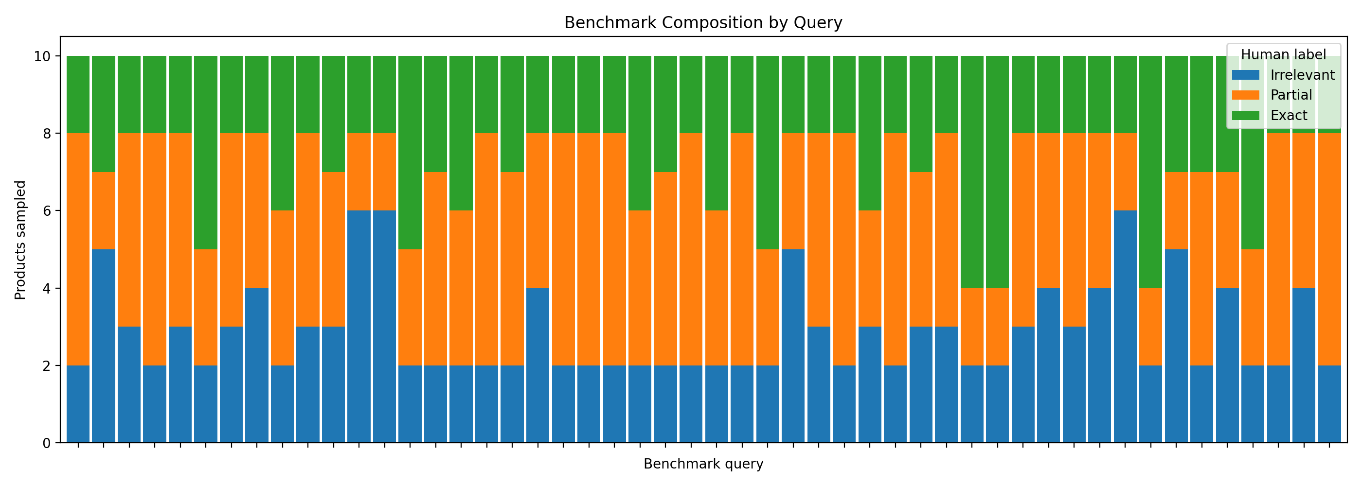
Figure 2. Benchmark composition by query. Each held-out query has a controlled mix of Irrelevant, Partial, and Exact products.

Building the training set

For training, I sampled from the remaining queries after removing the benchmark queries.

This produced 5,074 training rows from 429 training queries, with a cap of 12 products per query.

The training data was capped per query so that a few large queries would not dominate the dataset. I also tried to rebalance the labels so that Exact and Irrelevant examples were better represented than they were in the raw dataset.

Although I tried to rebalance the labels, the final training set was still Partial-heavy: about 48.9% Partial, 28.1% Irrelevant, and 23.0% Exact. The training distribution was close to the benchmark distribution, but still leaned more heavily toward Partial. That became important later: the fine-tuned model often preferred Partial over Exact.

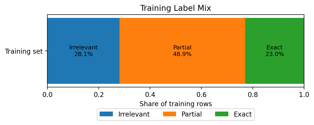
Figure 3. Final label mix in the training set after sampling. The training data remained Partial-heavy: 48.9% Partial, 28.1% Irrelevant, and 23.0% Exact.

Data validation

Before fine-tuning, I used a small split script to validate the instruction-tuning JSONL. It checked that every row had the required fields, that outputs were restricted to SCORE: 0, SCORE: 1, or SCORE: 2, deduplicated rows, and split train/eval data by query_id rather than arbitrary rows.

This mattered because query-level splitting reduces leakage. If the same query appears in both training and evaluation, the benchmark can look better than it really is.

Why this preparation mattered

The data preparation shaped the rest of the experiment.

The benchmark was a controlled test set for relevance judging. That made it useful for comparing LLM judges, but it also means the results should be interpreted carefully: this benchmark measures performance on a balanced, diagnostic WANDS subset, not on the raw WANDS distribution.

The question was whether a model could reliably tell the difference between Irrelevant, Partial, and Exact products when all three were present.

At this point I had two things: a compact training set for teaching the score format, and a separate 500-row benchmark for checking whether the trained model actually behaved better. The next step was to see whether a small model could learn the relevance rubric well enough to be useful inside judgement-ai.

Fine-tuning a local judge

After preparing the training and benchmark datasets, I wanted to test whether a small local model could learn the WANDS relevance rubric.

The task was narrow: given a search query and a candidate product, return one of three relevance scores.

SCORE: 0
SCORE: 1
SCORE: 2

I used unsloth/qwen3.5-4b-base as the base model. This was important because I was not starting from a polished instruction-following judge. The model had to learn both the relevance task and the strict output format from the fine-tuning data.

I trained the model in Google Colab using Unsloth Studio. Unsloth documents workflows for training models on Colab, Kaggle, or local machines, and its documentation describes QLoRA as combining LoRA with 4-bit precision to handle large models with fewer resources.³ Since I was working within the limits of a free Colab session, I used QLoRA rather than a full fine-tune. The goal was to see whether a practical local fine-tuning workflow could produce a useful search relevance judge.

The training setup stayed close to the defaults provided by Unsloth Studio:

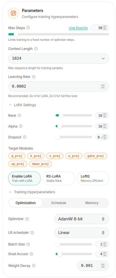
Figure 4. QLoRA training settings in Unsloth Studio. I mostly used the default configuration and limited training to one epoch.

The run completed after 620 steps, which corresponded to one epoch over the training set. I watched the training loss, evaluation loss, learning rate, and gradient norm during the run. The evaluation loss decreased early and then mostly flattened, so I did not treat the loss curve as proof that the model had become a reliable judge. The real test would be the held-out benchmark.

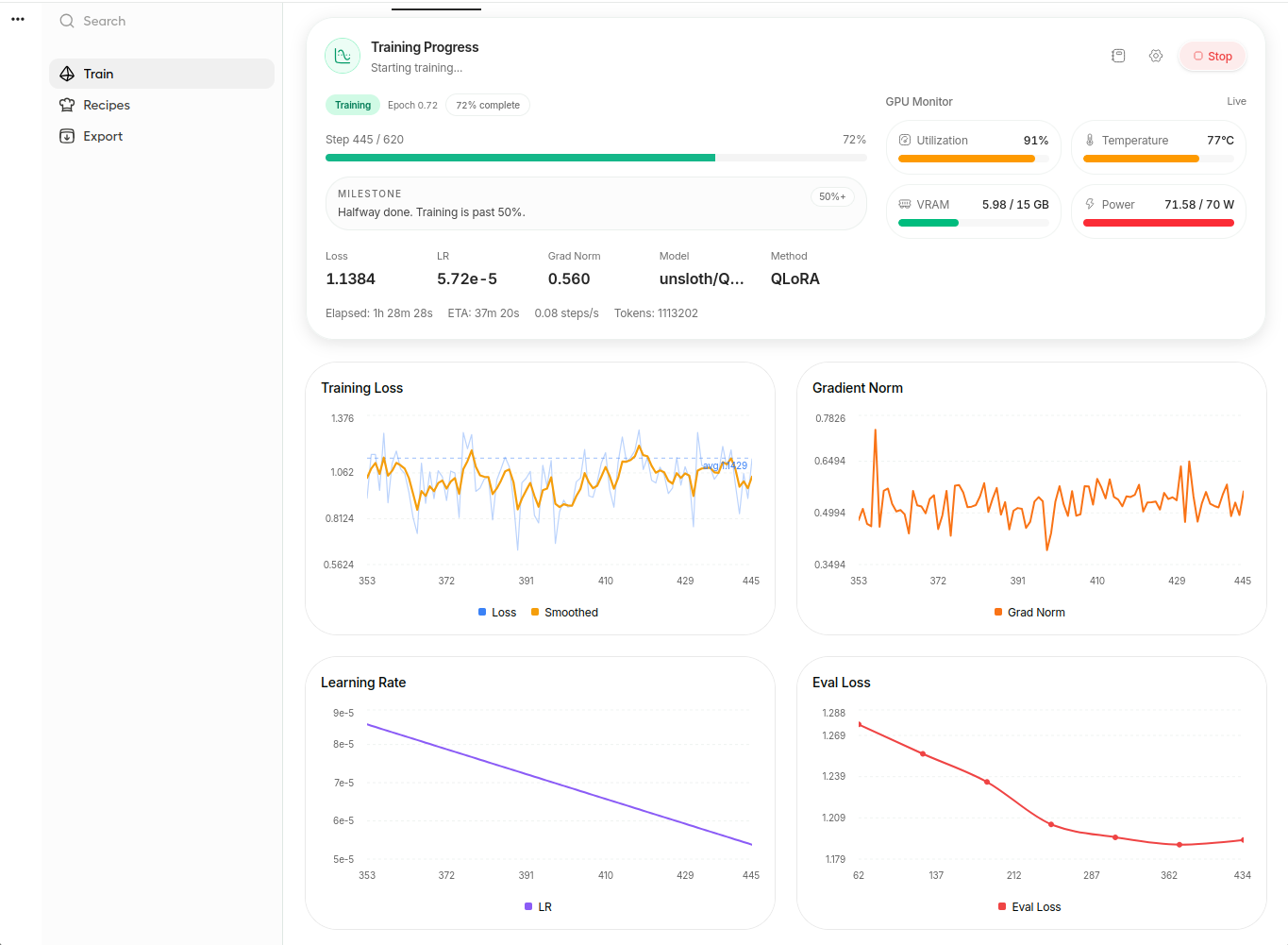
Figure 5. Training progress near the end of the run. The experiment used one epoch, no hyperparameter sweep, and a free Colab environment.

After training, I exported a merged bf16 model through the Hugging Face API. I then ran the fine-tuned model locally through Ollama. Ollama documents OpenAI-compatible API support, which is useful for tools that want to swap hosted and local models behind a similar interface.⁴ I used judgement-ai to generate relevance judgments on the 500-row benchmark; the tool is designed to grade query-document pairs with local or API-backed LLMs and save structured outputs for comparison.⁵

This part of the project exposed the practical limits of a single supervised fine-tuning run. There were many choices that could have changed the outcome: the base model, the train/benchmark split, the label distribution, context length, learning rate, number of epochs, LoRA rank, and even the exact prompt format.

I did not try to optimize all of those. The workflow I completed was:

WANDS dataset → prepared JSONL → QLoRA fine-tune → local Ollama model → judgement-ai benchmark → metric comparison

That made the result useful even though the fine-tuned model was not a human-level judge.

What the results were

After fine-tuning, I used judgement-ai to run the same 500-row benchmark across several judges:

• Qwen 3.5 4B instruct bf16
• fine-tuned Qwen 3.5 4B bf16
• GPT-5.5

One limitation is possible data contamination. WANDS is a public dataset, and modern LLM training corpora may include public GitHub repositories, papers, dataset mirrors, or derived examples. I cannot verify whether GPT-5.5 or Qwen saw WANDS during pretraining. Because of that, I treat these benchmark results as evidence of behavior on this dataset, not as proof of generalization to unseen relevance-judging tasks.

Each model produced one score per query-product pair, and I compared those scores against the original WANDS human labels.

Before showing the results, here is how I evaluated the judges.

Accuracy is the percentage of rows where the model exactly matched the WANDS human label.

Macro-F1 averages F1 across the three labels: Irrelevant, Partial, and Exact. F1 combines precision and recall, and macro-averaging gives each class equal weight instead of letting the largest class dominate the result.⁶

Quadratic weighted kappa measures agreement between the model and the human labels while accounting for agreement that could happen by chance. I used the quadratic version because the labels are ordered: confusing Irrelevant with Exact is worse than confusing Partial with one of its neighboring labels.⁷

As a rough interpretation guide, the Landis and Koch scale describes kappa values from 0.41–0.60 as moderate agreement, 0.61–0.80 as substantial agreement, and 0.81–1.00 as almost perfect agreement. I treat this as a guide rather than a strict cutoff.

MAE, or mean absolute error, treats the labels as ordinal scores. A prediction of 1 when the human label is 2 has an error of 1; a prediction of 0 when the human label is 2 has an error of 2.⁸

Severe error rate is the share of rows where the model made the largest possible mistake: predicting Exact for a human Irrelevant item, or predicting Irrelevant for a human Exact item.

Overall model performance

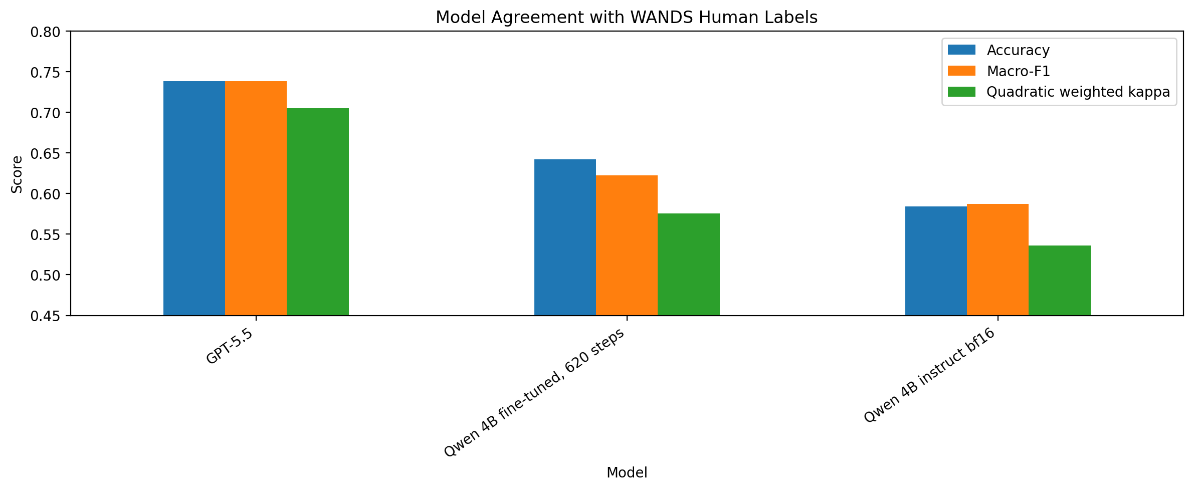
Figure 6. Agreement with WANDS human labels. The y-axis is narrowed to make differences easier to compare, so the visual gap should be read together with the numeric table below.

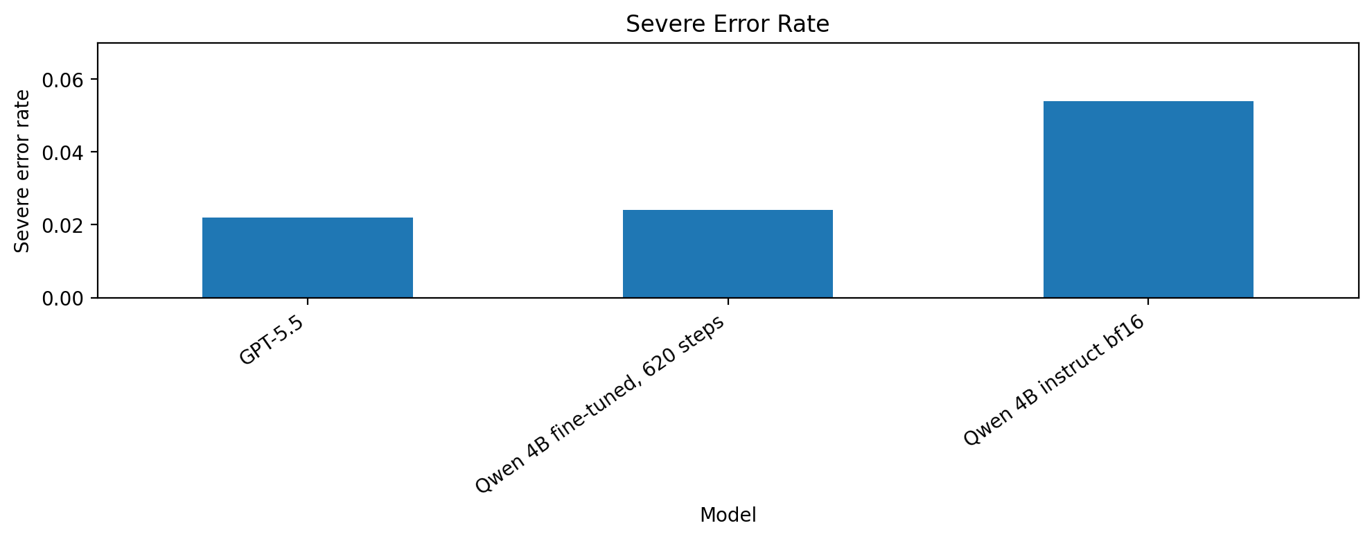
Figure 7. Severe error rate. Lower is better. A severe error means predicting Exact for a human Irrelevant item or Irrelevant for a human Exact item.

The strongest judge was GPT-5.5:

Model	Kappa	Accuracy	Macro-F1	Severe error	MAE
GPT-5.5	0.705	0.738	0.738	2.2%	0.284
Qwen 4B fine-tuned	0.576	0.642	0.623	2.4%	0.382
Qwen 4B instruct	0.536	0.584	0.587	5.4%	0.470

The fine-tuned Qwen model improved over the instruct Qwen model, but the improvement was not dramatic. The best fine-tuned run, qwen35-4b-bf16-wands620, improved accuracy from 0.584 to 0.642, macro-F1 from 0.587 to 0.623, and quadratic weighted kappa from 0.536 to 0.576.

The clearest improvement was in severe errors. I counted a severe error as a direct Irrelevant ↔ Exact mistake. The instruct Qwen model had a severe error rate of 5.4%, while the best fine-tuned model reduced that to 2.4%.

Agreement vs severe mistakes

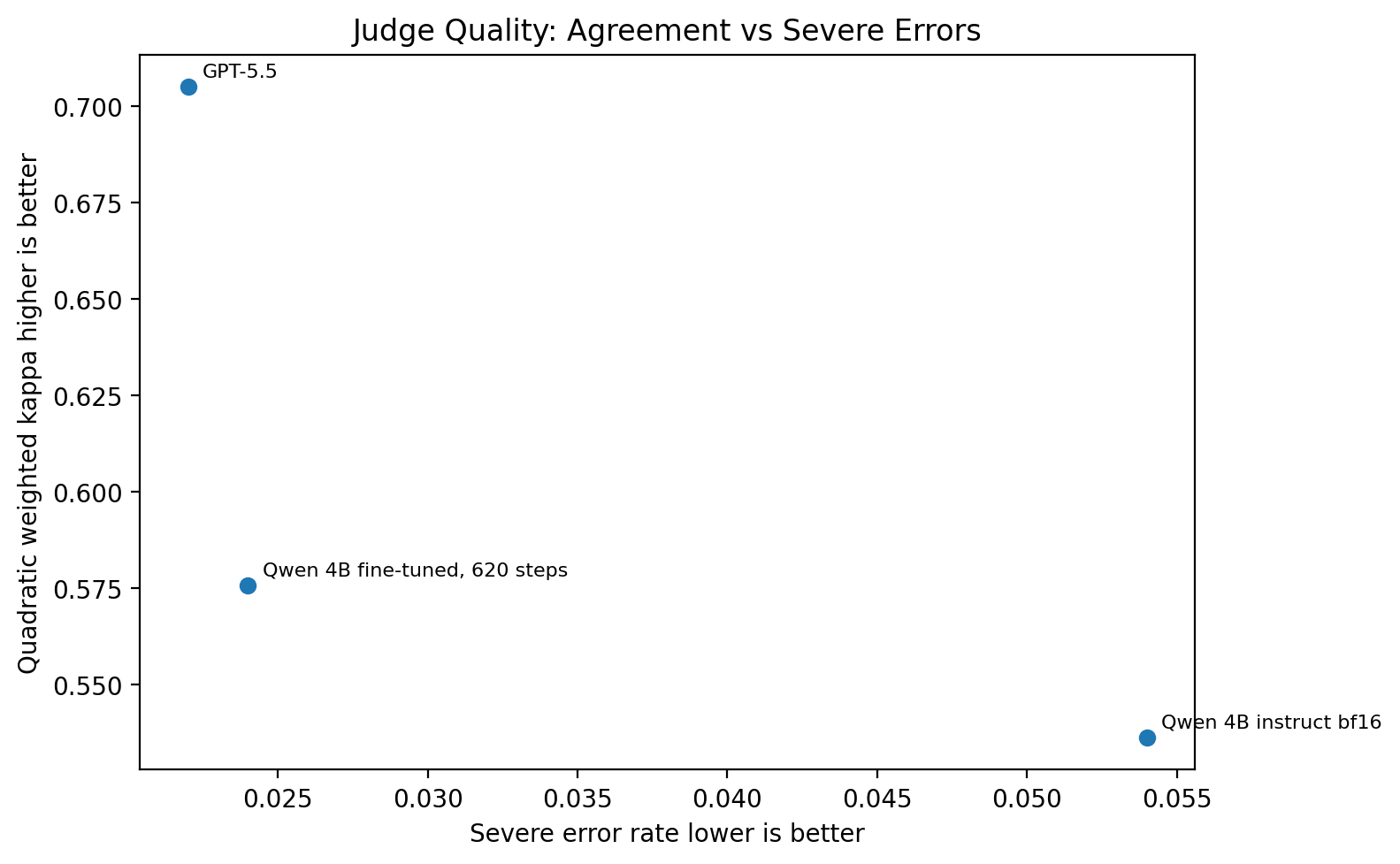
Figure 8. Judge quality as a tradeoff between agreement and severe mistakes. Better models are closer to the top-left.

This plot made the tradeoff easier to see. GPT-5.5 had the best overall agreement. The fine-tuned Qwen model did not reach GPT-5.5 quality, but it moved in the right direction compared with the instruct model: higher agreement and fewer severe mistakes.

What fine-tuning changed

For the label-level view, I used recall. Recall answers: among all rows that humans labeled as a class, how many did the model correctly recover? For example, Exact recall measures how often the model predicted Exact when the human label was actually Exact.

Precision answers the opposite question: among all rows the model predicted as a class, how many were correct? For example, Exact precision measures how trustworthy the model’s Exact predictions were.

The key pattern to watch is the Exact bar: the fine-tuned model improved on Irrelevant and Partial, but lost a lot of recall on Exact.

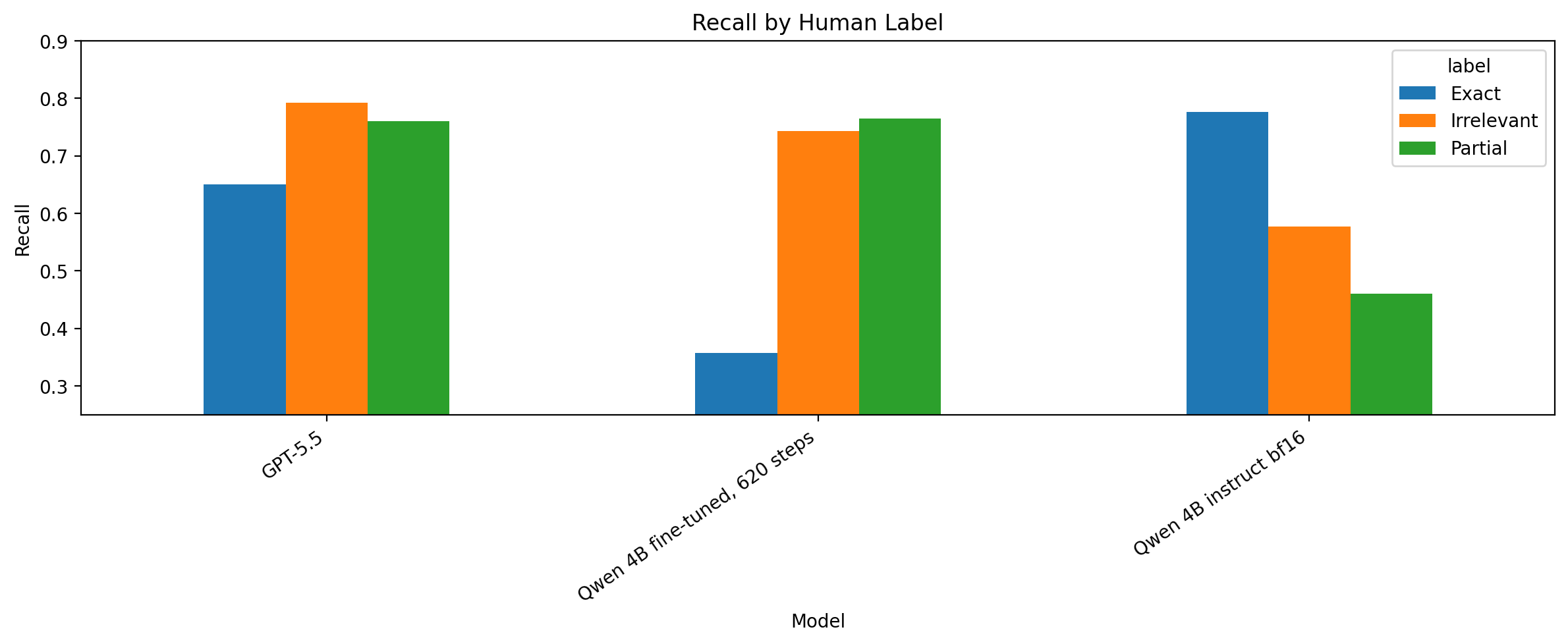
Figure 9. Recall by human label. The fine-tuned model became better at identifying Irrelevant and Partial examples, but weaker at confidently predicting Exact.

The class-level results were more useful than the headline metrics.

The fine-tuned model became more conservative. It was much less likely to call an irrelevant product exact, but it also became much less likely to call an exact product exact.

For the best fine-tuned model:

• Human Irrelevant → predicted Irrelevant: 74.3%
• Human Partial → predicted Partial: 76.5%
• Human Exact → predicted Exact: only 35.7%
• Human Exact → predicted Partial: 57.3%

So the model learned caution. It often recognized that an exact product was at least relevant, but downgraded it to Partial.

A confusion matrix shows where each human label ended up in the model predictions. The rows are human labels, and the columns are model predictions. The diagonal cells are correct predictions; the off-diagonal cells are mistakes.

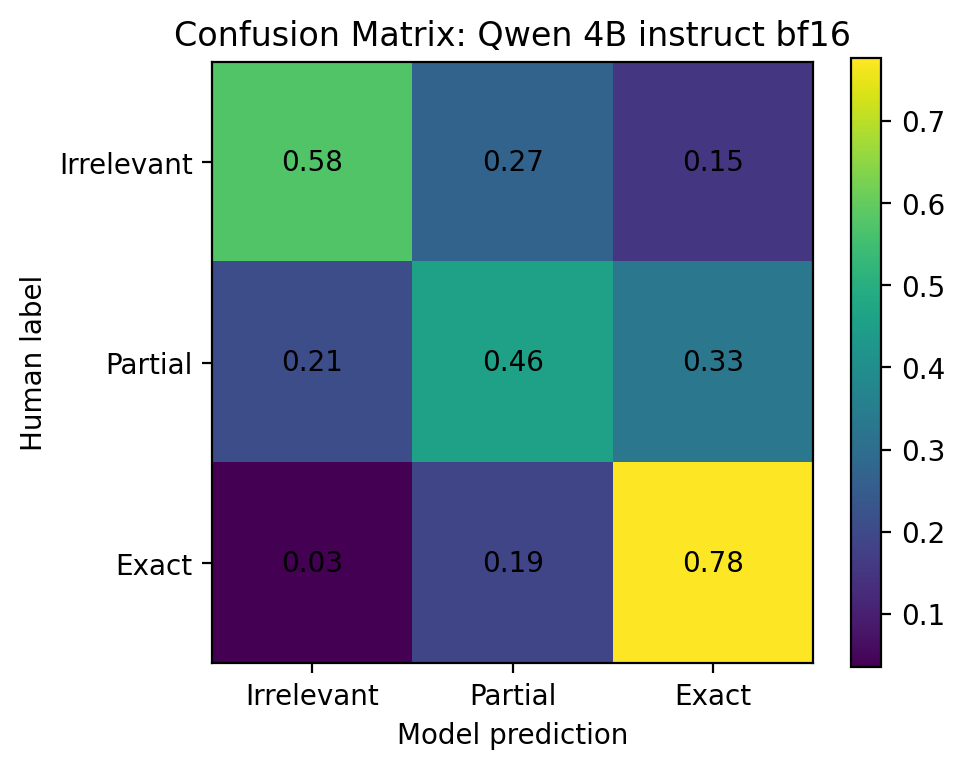
Figure 10. Qwen 3.5 4B instruct bf16 confusion matrix.

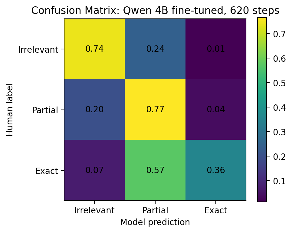
Figure 11. Fine-tuned Qwen confusion matrix. The model became safer, but less confident on Exact labels.

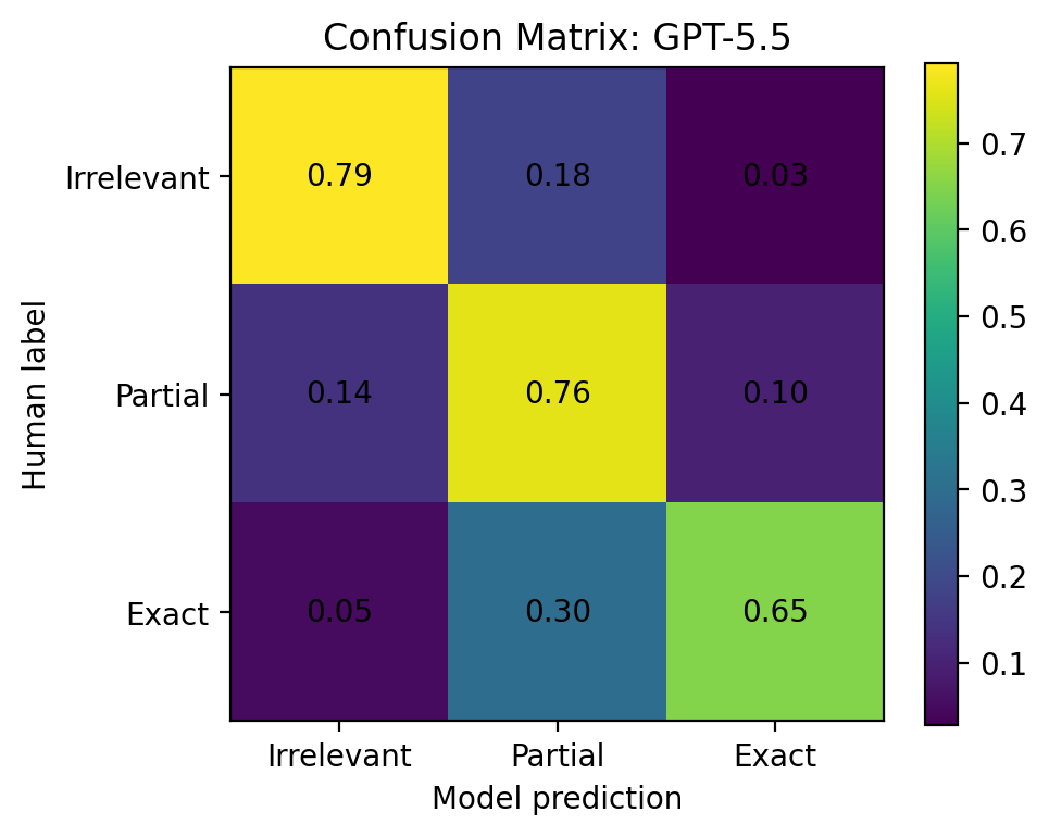
Figure 12. GPT-5.5 confusion matrix. GPT-5.5 was the most balanced judge in this benchmark.

Bootstrap confidence intervals

I also used query-level bootstrap confidence intervals. A bootstrap confidence interval repeatedly resamples the benchmark and recalculates the metric to estimate how much the result might move if the benchmark sample changed. I resampled by query rather than by row because the benchmark had 500 rows, but those rows came from only 50 queries. Rows from the same query are not fully independent.

The bootstrap results showed the same overall pattern:

Model	Accuracy CI	Kappa CI	Severe error CI
GPT-5.5	0.686–0.784	0.632–0.773	0.008–0.040
Qwen 4B fine-tuned, 620 steps	0.592–0.690	0.500–0.644	0.010–0.040
Qwen 4B instruct	0.524–0.648	0.451–0.626	0.032–0.078

This makes the result more cautious. The fine-tuned model improved in the raw metrics, especially on severe errors, but the confidence intervals are not wide enough to pretend this was a solved problem. The benchmark suggests the fine-tuned model moved in the right direction, especially on severe errors, but not enough to claim replacement-level reliability.

Conclusion

The fine-tuned model did not reach replacement-level reliability for human relevance judging.

It did improve over the instruct Qwen baseline. The strongest improvement was the reduction in severe Irrelevant ↔ Exact mistakes. That matters because those are the errors that would be most damaging in a relevance-grading workflow.

The tradeoff was that the model became conservative. It often downgraded human Exact examples to Partial. For a pre-labeling or triage workflow, that might be acceptable. For replacing human labels, it is not enough.

GPT-5.5 was still the strongest judge in this benchmark, but even it reached 0.705 quadratic weighted kappa rather than perfect agreement. That put the fine-tuning result in context: the task itself is messy, and WANDS-style relevance labels are not always easy to reproduce from product text alone.

The hardest part of the project was the number of decisions around the data and training setup: which base model to use, how to sample labels, how much to rebalance the dataset, how many epochs to train, how to write the prompt, and whether supervised fine-tuning is enough.

The next experiment I would run is much narrower: take the cases where the fine-tuned model predicted Partial but the human label was Exact, inspect them manually, and rebuild the training set around that failure mode. Before trying a more complex method like RL or preference training, I would want to know whether the model lacked examples, misunderstood the rubric, or learned the wrong bias from the sampling strategy.

The useful result from this work is the evaluation loop. judgement-ai gave me a way to run the same benchmark across local and hosted models, collect structured judgments, and compare those judgments against human labels. That turned model quality into something I could inspect instead of something I had to guess at.

References

1. Wayfair. “WANDS - Wayfair ANnotation Dataset.” GitHub. https://github.com/wayfair/WANDS ↩︎

2. Yan Chen, Shujian Liu, Zheng Liu, Weiyi Sun, Linas Baltrunas, and Benjamin Schroeder. “WANDS: Dataset for Product Search Relevance Assessment.” ECIR 2022. https://easychair.org/publications/preprint/j2D4/open ↩︎

3. Unsloth. “Fine-tuning LLMs Guide.” https://unsloth.ai/docs/get-started/fine-tuning-llms-guide ↩︎

4. Ollama. “OpenAI compatibility.” https://docs.ollama.com/api/openai-compatibility ↩︎

5. MclPio. “judgement-ai.” GitHub. https://github.com/MclPio/judgement-ai ↩︎

6. scikit-learn. “f1_score.” https://scikit-learn.org/stable/modules/generated/sklearn.metrics.f1_score.html ↩︎

7. scikit-learn. “cohen_kappa_score.” https://scikit-learn.org/stable/modules/generated/sklearn.metrics.cohen_kappa_score.html ↩︎

8. scikit-learn. “mean_absolute_error.” https://scikit-learn.org/stable/modules/generated/sklearn.metrics.mean_absolute_error.html ↩︎